Rendering Metaballs in 2D

Metaballs are blobby objects that "glue togheter" when they came close. They were Invented by Jim Blinn for the 1980 documentary TV show Cosmos to represent atoms and molecules. Metaballs later became a popular effect in the demoscene in the early 90s. In this article we'll see how render them in 2D.

If you're curious, there is a link in the References section to the original episode of Cosmos ¹ where the metaballs were used for the first time.

Isolines of a scalar field

Figure 1 show the output of the function of two variables:

$$f(x,y) = \frac{1}{r}$$

where r is the distance from the orgin, computed as $r=\sqrt{x^2+y^2}$. The higher values correspond to brighter pixels, which become darker as the distance from $(0,0)$ increases. The output of such a function is called a scalar field.

One scalar field	The metaball	Two fields summed	The metaball

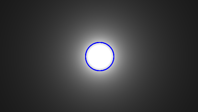Now we can define the metaball as:

The portion of the scalar field where its value is above a threshold.

Figure 2 shows in blue the pixels with the value of the threshold we choose, this is called an isoline. All the pixels inside the isolines are part of the metaball.

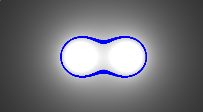
Translating the function slightly to the left and adding another one equal to it on its right (Figure 3), generate a scalar field that is the sum of both, and a new isoline.

Moving one function with respect to the other will result in a countinous change of the isolines, which "glue togher" when they came close, as shown in the following shader.

The falloff function

$f(x,y) = \frac{1}{r}$ is inversely proportional to the distance from the origin. For this reason we'll call it the falloff.

This particular funciton isn't the best choiche for some reasons:

• It's $+\infty$ in the origin, so we have to clamp it.
• There is a division that is expensive (at least on old hardware :))
• It never became zero, so we have always sum up all the functions to compute the field, no matter how far.

The following Desmos graph shows in the falloff in one dimension, as function of the distance from the origin $r$. In red the previous one and in blue the clamped version.

Actually we will use the green one, a cubic polynomial $f(r) = 1-(3r^2-2r^3)$, where $(3r^2-2r^3)$ is also known as the smoothstep function.

Using the cubic one we can ignore functions that are farther that the falloff lenght, avoid division and any discontinuity.

The lenght of the falloff can be changed by multipling the falloff argument by a value $a>0$ to increase the size of the metaballs, or $a<0$ to decrease it. (i.e. computing $f(ar)$);

ShaderToy code

Finally, here is the code that implement the previous shader, you can also click on the shader title and experiment directly in ShaderToy to see the result in real time. Comments have been added to explain the code in detail.

 1// This function is called for each pixel
 2void mainImage( out vec4 fragColor, in vec2 fragCoord)
 3{
 4    // Coordinated of the current pixel
 5    float x = fragCoord.x;
 6    float y = fragCoord.y;
 7    
 8    // In ShaderToy the point (0,0) is the bottom left angle,
 9    // but we want (0,0) at the center of the screen so translate it there.
10    vec2 Coord = (2.*fragCoord-iResolution.xy) / iResolution.y;
11    
12    // Scale up coordinates a little bit (zoom out)
13    Coord = Coord * 5.; 
14    
15    // Define the position of the two scalar fields
16    vec2 CHARGES_1_POS = vec2(2,0);
17    vec2 CHARGES_2_POS = vec2(-2,0);
18    
19    // Compute the first field value for this pixel 
20    float f1=0.;
21    CHARGES_1_POS.x *= 3.*sin(iTime);   // Move one of the two charges at each frame
22    float r1 = length(CHARGES_1_POS - Coord);
23    if(r1>3.) f1 = 0.;                  // Ouside the falloff, do not evaluate the function
24    f1 = 1.-smoothstep(0.,3.,r1); // Using 1-3x^2 - 2x^3 as falloff, that goes from 0 to 1 when r goes from 0 to 3 (scaled a little bit)
25    
26    // Compute the second field value for this pixel 
27    float f2=0.;
28    float r2 = length(CHARGES_2_POS - Coord);
29    if(r2>3.) f2 = 0.;                       // Ouside the falloff, do not evaluate the function
30    else f2 = 1.-smoothstep(0.,3.,r2); // Using 1-3x^2 - 2x^3 as falloff, that goes from 0 to 1 when r goes from 0 to 3 (scaled a little bit) 
31    
32    // Compute the sum of all fields
33    float fTotal = f1 + f2;
34    
35    // The surface of the metaball will be defined for the values less then 0.8.
36    // We'll show the isoline fTotal = 0.3, rendering the pixel that has
37    // fTotal value "near" 0.3 in blue
38    if(abs(fTotal-0.4) < 0.03)
39    {
40        fragColor = vec4(0,0,1,1);    
41    }
42    else 
43    {
44        fragColor = vec4(fTotal);
45    }
46}

Experiment

Now that we know the base effect, it's possible to add variations.

More fields and movements:

Or colors:

You can even experiment changing the falloff function. And more ...

This concludes our exploration of 2D metaballs. In the next article, we'll see how to render 3D metaballs!